Appearance
单因子研究报告:Piotroski F-Score(A股)· notebook 版
基本面强度评分(0~9)。本 notebook 含:因子构造、全市场横截面、有效性检验(IC/分层)、风格周期性。
复用已有缓存,完全离线:横截面读 results/fscore_2025.csv(run_fscore_scan.py 产出);有效性读 data/raw/fscore_raw_* 财报缓存 + fscore_bt_px.parquet 价格缓存 + fscore_hs300.parquet。
仅供研究学习,不构成投资建议。脚本版见
scripts/fscore_factor_report.py,实现见src/quant/factors/library/fscore.py。
python
%matplotlib inline
import os
while not os.path.exists("pyproject.toml") and os.getcwd() != "/":
    os.chdir("..")
import numpy as np, pandas as pd, matplotlib, matplotlib.pyplot as plt
from matplotlib import font_manager
for _n in ["PingFang SC", "Hiragino Sans GB", "Arial Unicode MS", "Songti SC"]:
    if _n in {f.name for f in font_manager.fontManager.ttflist}:
        matplotlib.rcParams["font.sans-serif"] = [_n]; break
matplotlib.rcParams["axes.unicode_minus"] = False

from quant.factors.library.fscore import SIGNAL_COLS, compute_fscore     # 内核:F-Score 计算

RAW = "data/raw"
SCAN_YEAR, BT_START, BT_END = 2025, 2015, 2024
SIGNAL_CN = {"f_roa": "ROA>0", "f_cfo": "经营现金流>0", "f_droa": "ROA同比上升",
             "f_accrual": "CFO>净利润(盈利质量)", "f_dlever": "长期负债率下降",
             "f_dliquid": "流动比率上升", "f_eqoffer": "未增发股本",
             "f_dmargin": "毛利率上升", "f_dturn": "资产周转率上升"}
scan_df = pd.read_csv("results/fscore_%d.csv" % SCAN_YEAR, index_col=0)
print("横截面(%d年报): 有效 %d 只, F-Score 均值 %.2f / 中位 %.0f; 高分(≥8) %d 只, 低分(≤1) %d 只" % (
    SCAN_YEAR, len(scan_df), scan_df["f_score"].mean(), scan_df["f_score"].median(),
    (scan_df["f_score"] >= 8).sum(), (scan_df["f_score"] <= 1).sum()))
横截面(2025年报): 有效 5589 只, F-Score 均值 4.95 / 中位 5; 高分(≥8) 431 只, 低分(≤1) 129 只
1. 因子构造
对每只股票取当年 t 与上年 t-1 年报,9 个“今年是否比去年变好”的判断,每项 1 分:
| # | 信号 | 记 1 分条件 | 组 |
|---|---|---|---|
| 1 | f_roa | ROA_t>0 | 盈利 |
| 2 | f_cfo | CFO_t>0 | 盈利 |
| 3 | f_droa | ROA_t>ROA_ | 盈利 |
| 4 | f_accrual | CFO_t>净利润_t(含金量) | 盈利 |
| 5 | f_dlever | 非流动负债率同比下降 | 杠杆 |
| 6 | f_dliquid | 流动比率同比上升 | 流动性 |
| 7 | f_eqoffer | 总股本 t≤t-1(未增发) | 融资 |
| 8 | f_dmargin | 毛利率同比上升 | 效率 |
| 9 | f_dturn | 资产周转率同比上升 | 效率 |
数据:tushare income/cashflow/balancesheet,合并报表、最新披露口径;缺字段→该信号记 0。
2. 全市场横截面(2025 年报)
python
dist = scan_df["f_score"].value_counts().reindex(range(10), fill_value=0).sort_index()
fig, ax = plt.subplots(figsize=(8.5, 4.4))
bars = ax.bar(dist.index.to_numpy(), dist.values, color="#3b6ea5")
bars[int(scan_df["f_score"].median())].set_color("#c0504d")
for x, c in zip(dist.index, dist.values):
    ax.text(x, c, str(int(c)), ha="center", va="bottom", fontsize=8)
ax.set_title("① 全市场 F-Score 分布(%d 年报,n=%d)" % (SCAN_YEAR, len(scan_df)))
ax.set_xlabel("F-Score(0~9)"); ax.set_ylabel("公司数"); ax.set_xticks(range(10))
ax.grid(axis="y", alpha=0.3); plt.show()

passrate = scan_df[SIGNAL_COLS].mean().sort_values(ascending=False)
print("各信号通过率(越低=该维度全市场普遍承压):")
for k, v in passrate.items():
    print("  %-12s %-22s %5.1f%%" % (k, SIGNAL_CN[k], v * 100))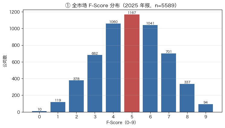
各信号通过率(越低=该维度全市场普遍承压):
  f_eqoffer    未增发股本                   75.8%
  f_roa        ROA>0                   73.5%
  f_cfo        经营现金流>0                 58.6%
  f_accrual    CFO>净利润(盈利质量)           52.6%
  f_dlever     长期负债率下降                 52.3%
  f_dturn      资产周转率上升                 47.2%
  f_dmargin    毛利率上升                   46.6%
  f_droa       ROA同比上升                 45.1%
  f_dliquid    流动比率上升                  43.6%
3. 有效性检验(2015~2024,年频,超额=个股−沪深300)
每年 5 月年报披露完毕调仓,持有一年,F-Score 与远期超额做 Spearman 秩相关与 10 档分层。
python
def _load_stmt(kind, period):
    df = pd.read_parquet("%s/fscore_raw_%s_%s.parquet" % (RAW, kind, period))
    df = df[df["report_type"].astype(str) == "1"].sort_values("ann_date")
    return df.drop_duplicates("ts_code", keep="last").set_index("ts_code")

def panel(period):
    inc, cf, bs = _load_stmt("income", period), _load_stmt("cashflow", period), _load_stmt("balancesheet", period)
    p = pd.DataFrame(index=inc.index)
    p["net_income"] = inc["n_income"]
    p["revenue"] = inc["revenue"].fillna(inc["total_revenue"])
    p["oper_cost"] = inc["oper_cost"]
    p["cfo"] = cf["n_cashflow_act"]
    for c in ("total_assets", "total_cur_assets", "total_cur_liab", "total_ncl", "total_share"):
        p[c] = bs[c]
    return p.astype(float)

idx = pd.read_parquet("%s/fscore_hs300.parquet" % RAW).set_index("trade_date")["close"]   # 沪深300(缓存)
px = pd.read_parquet("%s/fscore_bt_px.parquet" % RAW).pivot(
    index="trade_date", columns="ts_code", values="adjclose")
cal = idx.index.tolist()

def rb(y):
    aft = [d for d in cal if d >= "%d0501" % (y + 1)]
    return aft[0] if aft else None
rbm = {y: rb(y) for y in range(BT_START, BT_END + 2)}
rbm = {y: d for y, d in rbm.items() if d}
fsc = {y: compute_fscore(panel("%d1231" % y), panel("%d1231" % (y - 1)))["f_score"]
       for y in range(BT_START, BT_END + 1)}

recs, layers = [], {q: [] for q in range(10)}
for y in range(BT_START, BT_END + 1):
    d0, d1 = rbm.get(y), rbm.get(y + 1)
    if not d0 or not d1 or d0 not in px.index or d1 not in px.index:
        continue
    f = fsc[y].dropna()
    codes = [c for c in f.index if c in px.columns]
    r = px.loc[d1, codes] / px.loc[d0, codes] - 1.0
    bench = idx.loc[d1] / idx.loc[d0] - 1.0
    g = pd.DataFrame({"f": f.loc[codes], "exc": (r - bench).values}).dropna()
    if len(g) < 100:
        continue
    ic = g["f"].corr(g["exc"], method="spearman")
    q = pd.qcut(g["f"].rank(method="first"), 10, labels=False)
    ls = g["exc"][q == 9].mean() - g["exc"][q == 0].mean()
    for k in range(10):
        layers[k].append(g["exc"][q == k].mean())
    recs.append(dict(hold="%s→%s" % (d0[:6], d1[:6]), ic=ic, n=len(g), bench=bench, ls=ls))

val = pd.DataFrame(recs)
decile = pd.Series({k: np.nanmean(layers[k]) for k in range(10)})
icir = val["ic"].mean() / val["ic"].std()
ls_cum = float(np.cumprod(1.0 + val["ls"].fillna(0)).iloc[-1] - 1.0)
print("RankIC 均值 %.3f | ICIR %.2f | IC>0 占比 %.0f%% | 多空10年累计 %+.1f%%" % (
    val["ic"].mean(), icir, (val["ic"] > 0).mean() * 100, ls_cum * 100))
print("\n分层无单调性: Q1=%+.1f%% 反而 ≥ Q10=%+.1f%%(10档全正=市值效应,非因子alpha)" % (
    decile.iloc[0] * 100, decile.iloc[9] * 100))
RankIC 均值 0.024 | ICIR 0.46 | IC>0 占比 80% | 多空10年累计 -14.1%
分层无单调性: Q1=+3.9% 反而 ≥ Q10=+2.8%(10档全正=市值效应,非因子alpha)
python
fig, ax = plt.subplots(figsize=(9.2, 4.2))
ax.bar(range(len(val)), val["ic"].to_numpy(),
       color=["#2e7d32" if v > 0 else "#c0392b" for v in val["ic"]])
ax.axhline(0, color="k", lw=0.8)
ax.axhline(val["ic"].mean(), color="#888", ls="--", lw=1, label="均值 %.3f" % val["ic"].mean())
ax.set_xticks(range(len(val))); ax.set_xticklabels(val["hold"], rotation=45, ha="right", fontsize=8)
ax.set_title("② 逐年 RankIC(绿=正/红=负)— 2016~19 有效,2024~25 反转")
ax.set_ylabel("RankIC"); ax.legend(fontsize=8); ax.grid(axis="y", alpha=0.3); plt.show()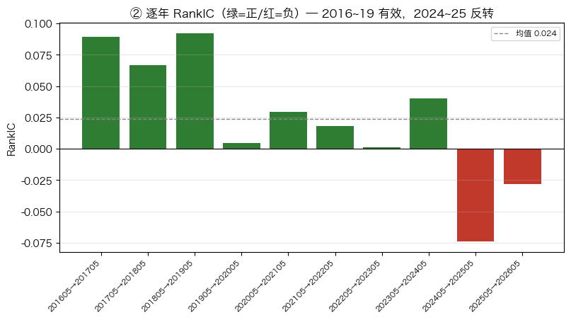
python
fig, (ax1, ax2) = plt.subplots(1, 2, figsize=(13, 4.2))
ax1.bar(range(10), (decile * 100).to_numpy(), color="#3b6ea5")
ax1.set_xticks(range(10)); ax1.set_xticklabels(["Q%d" % (k + 1) for k in range(10)])
ax1.set_title("③ 10 档年化超额(vs 沪深300)— 无单调性"); ax1.set_ylabel("年化超额 %")
ax1.grid(axis="y", alpha=0.3)

nav = np.cumprod(1.0 + val["ls"].fillna(0).to_numpy())
ax2.plot(range(len(nav)), nav, marker="o", ms=4, color="#6a4c93")
ax2.axhline(1.0, color="#888", ls="--", lw=1)
ax2.set_xticks(range(len(val))); ax2.set_xticklabels(val["hold"], rotation=45, ha="right", fontsize=8)
ax2.set_title("④ 多空(Q10-Q1)累计净值 — 十年原地踏步"); ax2.set_ylabel("累计净值")
ax2.grid(alpha=0.3); plt.show()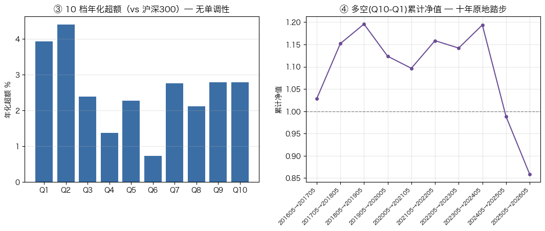
4. 风格周期性(关键发现)
python
def avg(years):
    m = val["hold"].str[:4].astype(int).isin(years)
    return val.loc[m, "ic"].mean()
r1, r2, r3 = avg(range(2016, 2020)), avg(range(2020, 2024)), avg(range(2024, 2027))
print("2016–2019 平均 RankIC %+.3f  价值·白马,质量有效 ✅" % r1)
print("2020–2023 平均 RankIC %+.3f  逐渐钝化" % r2)
print("2024–2025 平均 RankIC %+.3f  小盘/题材躁动,质量反转 ❌" % r3)
print("\nF-Score 是典型质量因子: 价值风格里有效,投机行情里反向。近两年负 IC 是连贯风格效应,非噪声。")
2016–2019 平均 RankIC +0.063 价值·白马,质量有效 ✅
2020–2023 平均 RankIC +0.022 逐渐钝化
2024–2025 平均 RankIC -0.051 小盘/题材躁动,质量反转 ❌
F-Score 是典型质量因子: 价值风格里有效,投机行情里反向。近两年负 IC 是连贯风格效应,非噪声。
5. 结论与使用建议
- 不要全市场裸用做多空:IC 仅 ~0.03、分层无梯度、多空近零。
- 回归 Piotroski 本意——价值域内二次筛子:先取低 PB/PE 一档,再在其中比高 F vs 低 F。
- 中性化:对市值/行业回归取残差,并用等权或市值匹配基准,剔除市值污染。
- 当质量过滤器:F-Score≤1 作基本面恶化预警,规避或剔出股票池。
- 严谨回测改 PIT:按
ann_date对齐,剔除最新披露口径下的重述前视。
裁决:❌ 全市场裸用偏弱(分层无单调性);✅ 但方向稳定、强风格周期性,应作“价值域内二次筛子”使用。